 |
ForecastingPro Description |
|
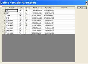
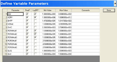
ForecastingPro® is the latest technology from NITEC for evaluation of uncertainty associated with prediction case scenarios in reservoir simulation. ForecastingPro uses defined uncertainties in reservoir and operating parameters and the simulation model to evaluate the probability of the performance results. The results are displayed as rate and cumulative production and injection profiles as a function of time for P10 through P90. ForecastingPro utilizes proprietary technology to assess the impact on forecasted field performance of an unlimited number of user defined reservoir and operating parameters over user specified ranges. The evaluation can be initiated at time zero (a Greenfield) or from history match run results from MatchingPro with their associated probabilities or from history match runs that have been made independent of MatchingPro. The process is completely automated once the user specifies the required parameters. ForecastingPro can currently interface with the Eclipse, Sensor and VIP simulators. Only Eclipse currently allows changes to reservoir parameters on a restart run. The ForecastingPro Process ForecastingPro needs very little information about the particulars of the prediction case or the reservoir being evaluated. Reservoir parameters and well and field data are only provided in the simulation data deck and need not be imported into ForecastingPro. The simulation data deck is treated as a template file which contains the user defined variable names for the uncertain parameters used in the analysis. These parameters must be identified along with the range over which they can vary. If this is a prediction study from an existing history match model, these parameters are typically those which do not have an impact on the history match period, but may have an impact on the predictions.
The user can identify a large number of uncertain reservoir and operating parameters (10 in this example), but choose to vary only a few in the analysis (7 in this example); others can be set to constant values. This provides the user with flexibility during the analysis process. ForecastingPro’s automated process uses distributed computing, hence it can take advantage of cluster servers and multiple CPUs to speed processing of the simulation runs required in the analysis. Once the user has identified the uncertain parameters to use in the analysis, the software determines the number of simulation runs that will be required to achieve reliable results. For more than five variables, testing has indicated that the number of simulation cases needed is 6 to 8 times the number of uncertain reservoir parameters being evaluated. (In this 7 parameter example, the maximum number of simulation runs is 43.) This is significantly fewer simulation runs than required by other software that rely on Latin Hypercube search methods for experimental design.
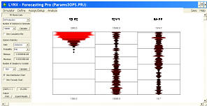
Once the auto process has completed the user can view the difference between the predicted performance of the response surface and the actual simulation run results for each run in a simple bar chart. Additional displays show the individual parameter variations in plots and charts. Again, recall that while a large number of uncertain parameters may be initially identified for analysis, the user can select any number for the analysis process.
The default frequency for the time interval used in the Monte Carlo analysis is annual. However, the user can select less frequent time periods to speed the analysis. Statistics in the form of distribution and Tornado charts can be displayed if desired. The user can then evaluate the statistics associated with any probability result at any of the specified times during the prediction. In this example, we choose the P90 results at 1/1/2025.
Selecting another point in time (1/1/2015)
for the same P90 results, the statistics can be displayed in a
Tornado chart. Unlike distribution plots, Tornado charts show
the sensitivity of results (cumulative oil recovery in this
case) to the uncertain parameters. As can be seen in
this example, the OWC parameter is still the most significant
parameter that impacts the results. Variation in the AQPV,
POROMult1 and AQJ parameters have less influence on the P90
results at this earlier point in time.
The green shading highlights -/+5% of the response range (oil recovery in this case) around the P90. Blue shading indicates that the derivative (i.e. dNp/dOWC) is positive (increases in the parameters value to the right increase the cumulative oil production; decreases to the left decrease the cumulative oil production). The red shading indicates that the derivative is negative (increases in the parameters value to the right decrease the cumulative oil production in this example).
An Operating Constraint Example The same example was run considering only variations in operating constraints. Three operating parameters and their ranges were added to the uncertain parameters list – BHPP (minimum well bottom hole production pressure), QLIQ (maximum well liquid production limit), and QWI (maximum well water injection limit). In the case of operating parameters, the term uncertainty is not appropriate. We should think in terms of variations in the parameter values instead.
|
 A
Greenfield Example
A
Greenfield Example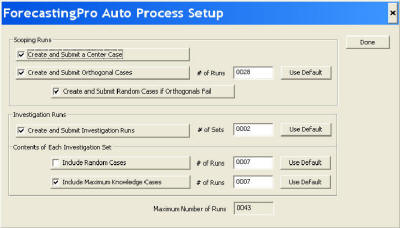 Proprietary
technology is used to develop an accurate response surface of
the simulated field performance of oil, water, and gas
production profiles, as well as gas and water injection
profiles. Initial experimental design (scoping) runs are
followed by a series of simulation (investigation) runs that
sequentially improve the ability of the response surface to
predict performance from any given set of uncertain
parameters. By default, all simulation prediction constraints
are honored in all simulation runs, hence the predicted
performance is only impacted by the perturbed parameters.
Proprietary
technology is used to develop an accurate response surface of
the simulated field performance of oil, water, and gas
production profiles, as well as gas and water injection
profiles. Initial experimental design (scoping) runs are
followed by a series of simulation (investigation) runs that
sequentially improve the ability of the response surface to
predict performance from any given set of uncertain
parameters. By default, all simulation prediction constraints
are honored in all simulation runs, hence the predicted
performance is only impacted by the perturbed parameters.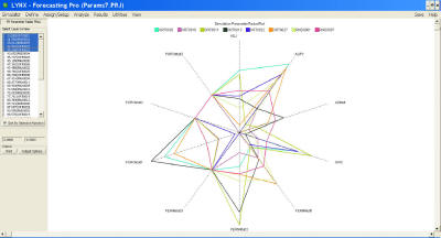 At
this point the response surface has been calibrated to the
actual simulation runs. To assess the performance profile for
any combination of parameters and the associated probability,
Monte Carlo analysis is used. The user can select any
combination of the parameters which have been varied or can
specify that some should have a specific value. The number of
Monte Carlo samples is input and the calculations are made. A
sample of 50,000 has been found to be generally satisfactory,
but a larger sample can be specified. This typically takes 30
seconds using a generic Windows personal computer.
At
this point the response surface has been calibrated to the
actual simulation runs. To assess the performance profile for
any combination of parameters and the associated probability,
Monte Carlo analysis is used. The user can select any
combination of the parameters which have been varied or can
specify that some should have a specific value. The number of
Monte Carlo samples is input and the calculations are made. A
sample of 50,000 has been found to be generally satisfactory,
but a larger sample can be specified. This typically takes 30
seconds using a generic Windows personal computer.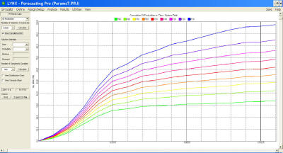 Once
the calculations have been made a cumulative performance
profile (oil, water, gas production and gas, water injection)
is available for display. P10 through P90 results are shown at
10 percent increments. Rate profiles are also available.
Once
the calculations have been made a cumulative performance
profile (oil, water, gas production and gas, water injection)
is available for display. P10 through P90 results are shown at
10 percent increments. Rate profiles are also available.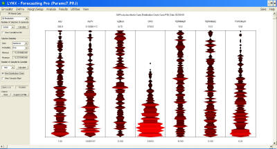 This
distribution plot displays a statistical likelihood
distribution of the 7 uncertain parameters for the selected
probability and time. It indicates that for the P90 case in
this example, the OWC parameter is likely to be at the low
range (shallow value). Among the other parameters, the
distribution of the AQPV, POROMult1 and AQJ also are likely to
be somewhat skewed. The remaining three parameters can be
practically any value within their ranges.
This
distribution plot displays a statistical likelihood
distribution of the 7 uncertain parameters for the selected
probability and time. It indicates that for the P90 case in
this example, the OWC parameter is likely to be at the low
range (shallow value). Among the other parameters, the
distribution of the AQPV, POROMult1 and AQJ also are likely to
be somewhat skewed. The remaining three parameters can be
practically any value within their ranges.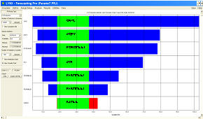
 In
this example, all of the other uncertain reservoir parameters
were set to constant values selected by the user. The
process of developing a reliable response surface required 19
simulation runs for the 3 operating parameters. Monte Carlo
analysis on the cumulative oil production and the associated
probabilities resulted in the display below.
In
this example, all of the other uncertain reservoir parameters
were set to constant values selected by the user. The
process of developing a reliable response surface required 19
simulation runs for the 3 operating parameters. Monte Carlo
analysis on the cumulative oil production and the associated
probabilities resulted in the display below.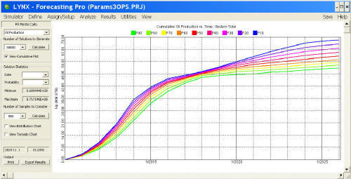
 Evaluation
of the P90 results (low cumulative oil production) at 1/1/2026
(end of the runs) using the Distribution plots shows that the
QLIQ must be in the higher range to yield the P90 results. The
other two operating parameters have little impact on
sensitivity of the results.
Evaluation
of the P90 results (low cumulative oil production) at 1/1/2026
(end of the runs) using the Distribution plots shows that the
QLIQ must be in the higher range to yield the P90 results. The
other two operating parameters have little impact on
sensitivity of the results.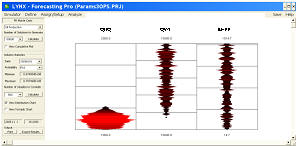 Accordingly,
evaluation of the P10 results (high cumulative oil production)
at the same time using the Distribution plots shows that the
QLIQ need only to be in the lower range to achieve the
reported results. Again, there is little sensitivity to
the other operating parameters.
Accordingly,
evaluation of the P10 results (high cumulative oil production)
at the same time using the Distribution plots shows that the
QLIQ need only to be in the lower range to achieve the
reported results. Again, there is little sensitivity to
the other operating parameters.